Machine Learning

Confusion Matrix

Confusion matrices help evaluate classification models by showing the true positives, false positives, true negatives, and false negatives.

The following example creates a confusion matrix between two vectors, simulating predicted and actual values:

from sklearn.metrics import confusion_matrix

tn, fp, fn, tp = confusion_matrix([0, 1, 0, 1], [1, 1, 1, 0]).ravel()
(tn, fp, fn, tp)

True Negatives (TN): Cases where the model correctly predicted 0. (In this case 0.)
False Positives (FP): Cases where the model incorrectly predicted 1 when it was actually 0. (In this case 2.)
False Negatives (FN): Cases where the model incorrectly predicted 0 when it was actually 1. (In this case 1.)
True Positives (TP): Cases where the model correctly predicted 1. (In this case 1.)

For real-world scenarios, confusion matrices provide insights into classification errors, as shown below:

import matplotlib.pyplot as plt
from sklearn.datasets import make_classification
from sklearn.metrics import confusion_matrix, ConfusionMatrixDisplay
from sklearn.model_selection import train_test_split
from sklearn.svm import SVC

X, y = make_classification(random_state=0)
X_train, X_test, y_train, y_test = train_test_split(X, y, random_state=0)
clf = SVC(random_state=0)
clf.fit(X_train, y_train)

predictions = clf.predict(X_test)
cm = confusion_matrix(y_test, predictions, labels=clf.classes_)
disp = ConfusionMatrixDisplay(confusion_matrix=cm, display_labels=clf.classes_)
disp.plot()
plt.show()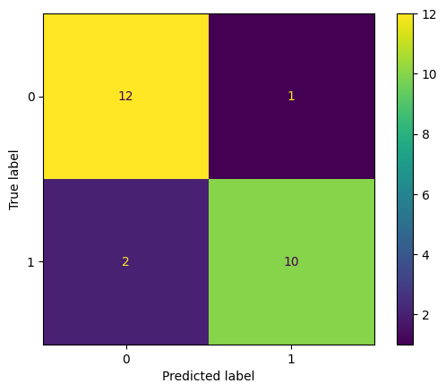

Linear Regression

F1, Accuracy, Recall, AUC, and Precision Scores

F1 Score

The F1 score is the harmonic mean of precision and recall, balancing their trade-offs. It’s particularly useful for imbalanced datasets.

from sklearn.metrics import f1_score

y_true = [0, 1, 2, 0, 1, 2]
y_pred = [0, 2, 1, 0, 0, 1]

print(f"Macro F1: {f1_score(y_true, y_pred, average='macro')}")
print(f"Micro F1: {f1_score(y_true, y_pred, average='micro')}")
print(f"Weighted F1: {f1_score(y_true, y_pred, average='weighted')}")
print(f"No Average F1: {f1_score(y_true, y_pred, average=None)}")

Macro F1: 0.26666666666666666
Micro F1: 0.3333333333333333
Weighted F1: 0.26666666666666666
No Average F1: [0.8 0.  0. ]

Accuracy

Accuracy is the ratio of correctly predicted observations to total observations.

from sklearn.metrics import accuracy_score

y_pred = [0, 2, 1, 3]
y_true = [0, 1, 2, 3]
accuracy_score(y_true, y_pred)

2/4 = 0.5

Precision

Precision is the ratio of true positives to the sum of true positives and false positives. So even if we have a low accuracy, precision que be maximal as in the following example:

from sklearn.metrics import precision_score

y_pred = [0, 1, 0, 0]
y_true = [0, 1, 1, 1]
precision_score(y_true, y_pred)

1/1 = 1

If in a multiclass scenario, the average is taken.

y_true = [0, 1, 2, 0, 1, 2]
y_pred = [0, 2, 1, 0, 0, 1]
precision_score(y_true, y_pred, average='macro')

0.2222222222222222

Recall

Recall is the ratio of true positives to the sum of true positives and false negatives.

from sklearn.metrics import recall_score

y_true = [0, 1, 2, 0, 1, 2]
y_pred = [0, 2, 1, 0, 0, 1]
recall_score(y_true, y_pred, average='macro')

0.3333333333333333

Classification Report

Provides a comprehensive overview of precision, recall, F1 score, and support.

from sklearn.metrics import classification_report

y_true = [0, 1, 2, 2, 2]
y_pred = [0, 0, 2, 2, 1]
target_names = ['class 0', 'class 1', 'class 2']
print(classification_report(y_true, y_pred, target_names=target_names))

precision    recall  f1-score   support

     class 0       0.50      1.00      0.67         1
     class 1       0.00      0.00      0.00         1
     class 2       1.00      0.67      0.80         3

    accuracy                           0.60         5
   macro avg       0.50      0.56      0.49         5
weighted avg       0.70      0.60      0.61         5

AUC (Area Under the Curve)

from sklearn.datasets import load_breast_cancer
from sklearn.linear_model import LogisticRegression
from sklearn.metrics import roc_auc_score

X, y = load_breast_cancer(return_X_y=True)
clf = LogisticRegression(solver="liblinear", random_state=0).fit(X, y)
roc_auc_score(y, clf.predict_proba(X)[:, 1])

Regression Metrics

RMSE (Root Mean Square Error)

Evaluates the standard deviation of prediction errors.

from sklearn.metrics import mean_squared_error

y_true = [3, -0.5, 2, 7]
y_pred = [2.5, 0.0, 2, 8]
mean_squared_error(y_true, y_pred)

MAE (Mean Absolute Error)

Measures average magnitude of errors in predictions.

from sklearn.metrics import mean_absolute_error

y_true = [3, -0.5, 2, 7]
y_pred = [2.5, 0.0, 2, 8]
mean_absolute_error(y_true, y_pred)

R Squared (Coefficient of Determination)

Explains the proportion of variance in the dependent variable that is predictable.

from sklearn.metrics import r2_score

y_true = [3, -0.5, 2, 7]
y_pred = [2.5, 0.0, 2, 8]
r2_score(y_true, y_pred)

Model Performance Measurement