CNN Model Activity

The following project was provided as part of Unit 9 and focuses on object recognition tasks using Convolutional Neural Networks (CNNs). The primary objective was to implement the code, analyze the results, and reflect on its components. The methods demonstrated here will be foundational for tasks in later units. You can refer to Unit 11 here for the personalized inplementation of this code for the final project.

Find below relevant snippets of the codes and my reasoning and understanding of each of the components.

---

Data Exploration

Viewing the Dataset

Exploring the dataset visually was essential for understanding its structure. Each image is 32×32×3, where the dimensions represent width, height, and RGB color channels. This was probably the most complex data dimension we have worked with so far.

# Displaying the first image using IPython display
pic = array_to_img(x_train_all[0])
display(pic)

# Displaying the first image using Matplotlib
plt.imshow(x_train_all[0])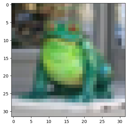

---

Data Preprocessing

In order for the model to learn from the data provided, we need to ensure that the information is not only in the correct format but also transformed or simplified to allow the model to use it optimally.

Scaling the Input Data

Scaling pixel values to the range [0, 1] ensures numerical stability during training and helps the model converge faster. Raw pixel values range from 0 to 255, so dividing by 255 standardizes them into a more manageable magnitude.

x_train_all = x_train_all / 255.0
x_test = x_test / 255.0

Categorical Encoding of Labels

Since we have 10 classes, converting the labels to categorical format enables the model to compute probabilities for each class during classification. Note the difference between having the output as a magnitude ranging from 0 to 10, versus having 10 labels named 1-10.

y_cat_train_all = to_categorical(y_train_all, 10)
y_cat_test = to_categorical(y_test, 10)

Creating Validation Dataset

Splitting the training data into training and validation subsets ensures that the model can be evaluated on unseen data during training. This approach helps detect overfitting early. We will dive into this concept again during Unit 11.

VALIDATION_SIZE = 10000
x_val = x_train_all[:VALIDATION_SIZE]
y_val_cat = y_cat_train_all[:VALIDATION_SIZE]

x_train = x_train_all[VALIDATION_SIZE:]
y_cat_train = y_cat_train_all[VALIDATION_SIZE:]

---

Model Building

Creating the CNN Model

The proposed architecture consists of two convolutional layers, each followed by max-pooling, to capture spatial hierarchies. A dense layer with 256 neurons is added for representation learning, followed by a softmax layer for multi-class classification.

model = Sequential()

# First Convolutional Layer
model.add(Conv2D(filters=32, kernel_size=(4,4), input_shape=(32, 32, 3), activation='relu'))
model.add(MaxPool2D(pool_size=(2, 2)))

# Second Convolutional Layer
model.add(Conv2D(filters=32, kernel_size=(4,4), activation='relu'))
model.add(MaxPool2D(pool_size=(2, 2)))

# Flattening and Dense Layers
model.add(Flatten())
model.add(Dense(256, activation='relu'))
model.add(Dense(10, activation='softmax'))

# Compiling the Model
model.compile(loss='categorical_crossentropy', optimizer='adam', metrics=['accuracy'])

For this particular activity I left the model as is, and really focused on the dimensionallity change across layers, as seen below.

Model Summary

Layer (type)	Output Shape	Param #
conv2d (Conv2D)	(None, 29, 29, 32)	1,568
max_pooling2d (MaxPooling2D)	(None, 14, 14, 32)	0
conv2d_1 (Conv2D)	(None, 11, 11, 32)	16,416
max_pooling2d_1 (MaxPooling2D)	(None, 5, 5, 32)	0
flatten (Flatten)	(None, 800)	0
dense (Dense)	(None, 256)	205,056
dense_1 (Dense)	(None, 10)	2,570

As we can see, each of the convolutional layers are reducing the dimensionallity, as we are no forcing them to keep the original size. Equally is done by the max-pooling layers which simplify the output of the convolutional layers to provide a high level overview of the learned features. The dense layers converge all the information into a one-dimensional vector which is eventually reduced to size 10, with a probability for each of the classes.

---

Training the Model

Early Stopping

During training, I would like to highlight the Early Stopping mechanism. It monitors the validation loss during training and stops the process if no improvement is observed for a specified number of epochs. This prevents overfitting and saves computational resources. In this particular case, if the validation loss did not improve for two consecutive epochs, the trainign is stoped.

from tensorflow.keras.callbacks import EarlyStopping

# Setting up Early Stopping
early_stop = EarlyStopping(monitor='val_loss', patience=2)

# Training the Model
history = model.fit(x_train, y_cat_train, epochs=25, validation_data=(x_val, y_val_cat), callbacks=[early_stop])

Training and Validation Metrics

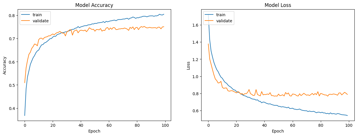
The main take away from training was to really visualize how to losses decreased for both the datasets and when the model decided to stop. In the following plot we can see the results for higher patience values. Where the validation loss did not improve and the model began overfitting.

---

Model Evaluation

Evaluating on the test set provides a realistic measure of how the model performs on unseen data.

Classification Report and Confusion Matrix

The classification report includes precision, recall, and F1-score, providing a detailed view of the model’s performance for each class.

Class	Precision	Recall	F1-score	Support
0	0.79	0.77	0.78	1000
1	0.84	0.89	0.87	1000
2	0.72	0.66	0.69	1000
3	0.55	0.59	0.57	1000
4	0.75	0.70	0.73	1000
5	0.64	0.67	0.66	1000
6	0.82	0.84	0.83	1000
7	0.86	0.80	0.83	1000
8	0.81	0.89	0.85	1000
9	0.83	0.81	0.82	1000
Accuracy			0.76	10000
Macro avg	0.76	0.76	0.76	10000
Weighted avg	0.76	0.76	0.76	10000

The confusion matrix visualizes correct and incorrect predictions.

	0	1	2	3	4	5	6	7	8	9
0	765	21	44	18	17	5	3	9	87	31
1	13	889	1	6	2	2	4	1	26	56
2	59	6	656	71	60	55	46	18	19	10
3	14	16	49	591	57	165	53	23	17	15
4	22	5	53	76	704	41	49	36	11	3
5	10	2	41	176	39	668	16	25	8	15
6	6	2	28	71	18	23	836	2	9	5
7	12	2	26	36	40	64	8	796	4	12
8	38	27	10	4	1	6	3	0	888	23
9	32	84	6	18	4	7	1	11	29	808

---

Predicting on Single Image

Visualizing individual predictions allows us to verify the model’s accuracy for specific examples. This step is especially interesting to visualize the results in a visual manner.

from random import randint

idx = randint(0, len(x_test)-1)

test_image = x_test[idx]

plt.imshow(test_image)
plt.show()

print(f"Real Label: {CLASS_NAMES[y_test_multiclass[idx]]}")
print(f"Predicted Label: {CLASS_NAMES[predictions[idx]]}")

Real Label: Frog
Predicted Label: Frog

---

Overall this was an excelent activity to really grasp on the concepts of neural networks and visualize the results of a simple use case.